
VAE: giving your Autoencoder the power of imagination
We will take a detailed look at the Variational Autoencoder: a generative model based on its more commonplace sibling, the Autoencoder (which we will devote some time to below as well).

We just released GPU Instances, our first servers equipped with graphical processing units (GPUs). Powered by high-end 16-GB NVIDIA Tesla P100 cards and highly efficient Intel Xeon Gold 6148 CPUs, they are ideal for data processing, artificial intelligence, rendering, and video encoding. In addition to the dedicated GPU and 10 Intel Xeon Gold cores, each instance comes with 45 GB of memory, 400 GB of local NVMe SSD storage, and is billed €1 per hour or €500 per month.
Today, we present you with a concrete use case for GPU Instances using deep learning to obtain a frontal rendering of facial images. Feel free to try it too. To do so, visit the Scaleway console to ask for quotas before creating your first GPU Instance.
Graphical processing unit (GPU) became a go-to term for the specialized electronic circuit designed to power graphics on a machine in the late 1990s, when it was popularized by the chip manufacturer NVIDIA.
GPUs were originally produced primarily to drive high-quality gaming experiences, producing life-like digital graphics. Today, those capabilities are being harnessed more broadly to accelerate computational workloads in areas such as artificial intelligence, machine learning and complex modeling.
GPU Instances at Scaleway were designed to be optimized for taking huge batches of data and performing the same operation over and over very quickly. The combination of an efficient CPU with a powerful GPU will deliver the best value of system performance and price for your deep learning applications.
Screenwriters never cease to amuse us with bizarre portrayals of the tech industry, ranging from cringeworthy to hilarious. With the current advances in artificial intelligence, however, some of the most unrealistic technologies from the TV screens are coming to life.
For example, the Enhance software from CSI: NY (or Les Experts : Manhattan for our francophone readers) has already been outshone by the state-of-the-art Super Resolution neural networks. On a more extreme side of the imagination, there is Enemy of the state:
“Rotating [a video surveillance footage] 75 degrees around the vertical” must have seemed completely nonsensical long after 1998 when the movie came out, evinced by the YouTube comments below this particular excerpt:

Despite the apparent pessimism of the audience, thanks to machine learning today anyone with a little bit of Python knowledge, a large enough dataset, and a Scaleway account can take a stab at writing a sci-fi drama worthy program.
Forget MNIST, forget the boring cat vs. dog classifiers, today we are going to learn how to do something far more exciting! This article is inspired by the impressive work by R. Huang et al. (Beyond Face Rotation: Global and Local Perception GAN for Photorealistic and Identity Preserving Frontal View Synthesis), in which the authors synthesise frontal views of people’s faces given their images at various angles.
We are not going to try to reproduce the state-of-the-art model by R. Huang et al. You will learn:
DALI library for highly optimized pre-processing of images on the GPU and feeding them into a deep learning model.PyTorchYou will also have your very own Generative Adversarial Network set up to be trained on a dataset of your choice. Without further ado, let’s dig in!
If you have not already gotten yourself a GPU instance hosted by Scaleway, you may do so by:
Compute tab on the left sidebar and clicking on the green + Create a server button.GPU OS in Choose an Image and GPU in Select a Server.For this project, feel free to choose either of the two GPU OS images currently available (10.1 and 9.2 refer to the corresponding versions of CUDA) and select RENDER-S as your server.

4 . Click on the green Create a new server button at the bottom of the page, and within seconds, your very own GPU Instance will be up and running!

5 . You can now ssh to it using the IP Address that you read off your list of instances under the Compute tab:
ssh root@[YOUR GPU INSTANCE IP ADDRESS]Docker way:If you are familiar with Docker, a convenient containerization platform that allows to package up applications together with all their dependencies, go ahead and pull our Docker image containing all the packages and the code needed for the Frontalization project, as well as a small sample dataset:
nvidia-docker run -it rg.fr-par.scw.cloud/opetrova/frontalization:tutorialroot@b272693df1ca:/Frontalization# lsDockerfile data.py main.py network.py test.py training_set(Note that you have to use nvidia-docker rather than the regular docker command due to the presence of a GPU.) You are now inside the Frontalization directory containing the four Python files whose contents we’ll go over below, and the training_set directory containing a sample training dataset. Great start, you can now proceed to Step 2!
If you are not familiar with Docker, no problem, you can easily set up the environment by hand. Scaleway GPU instances come with CUDA, Python and conda already installed, but at the time of writing, you have to downgrade the Python version to Python 3.6 in order for Nvidia’s DALI library to function:
conda install -y python==3.6.7conda install -y pytorch torchvisionpip install --extra-index-url https://developer.download.nvidia.com/compute/redist nvidia-dali==0.6.1You can upload your own training set onto your GPU instance via:
scp -r path/to/local/training_set root@[YOUR GPU INSTANCE IP ADDRESS]:/root/Frontalizationand save the Python code that you will see below inside the Frontalization directory using your terminal text editor of choice (e.g. nano or vim, both of which are already installed). Alternatively, you may clone Scaleway’s GitHub repository for this project.
At the heart of any machine learning project, lies the data. Unfortunately, Scaleway cannot provide the CMU Multi-PIE Face Database that we used for training due to copyright, so we shall proceed assuming you already have a dataset that you would like to train your model on. In order to make use of NVIDIA Data Loading Library (DALI), the images should be in.webp format. The dimensions of the images do not matter, since we have DALI to resize all the inputs to the input size required by our network (128×128 pixels), but a 1:1 ratio is desirable in order to obtain the most realistic synthesised images.
The advantage of using DALI over, e.g., a standard PyTorch Dataset, is that whatever pre-processing (resizing, cropping, etc.) is necessary, is performed on the GPU rather than the CPU, after which pre-processed images on the GPU are fed straight into the neural network.
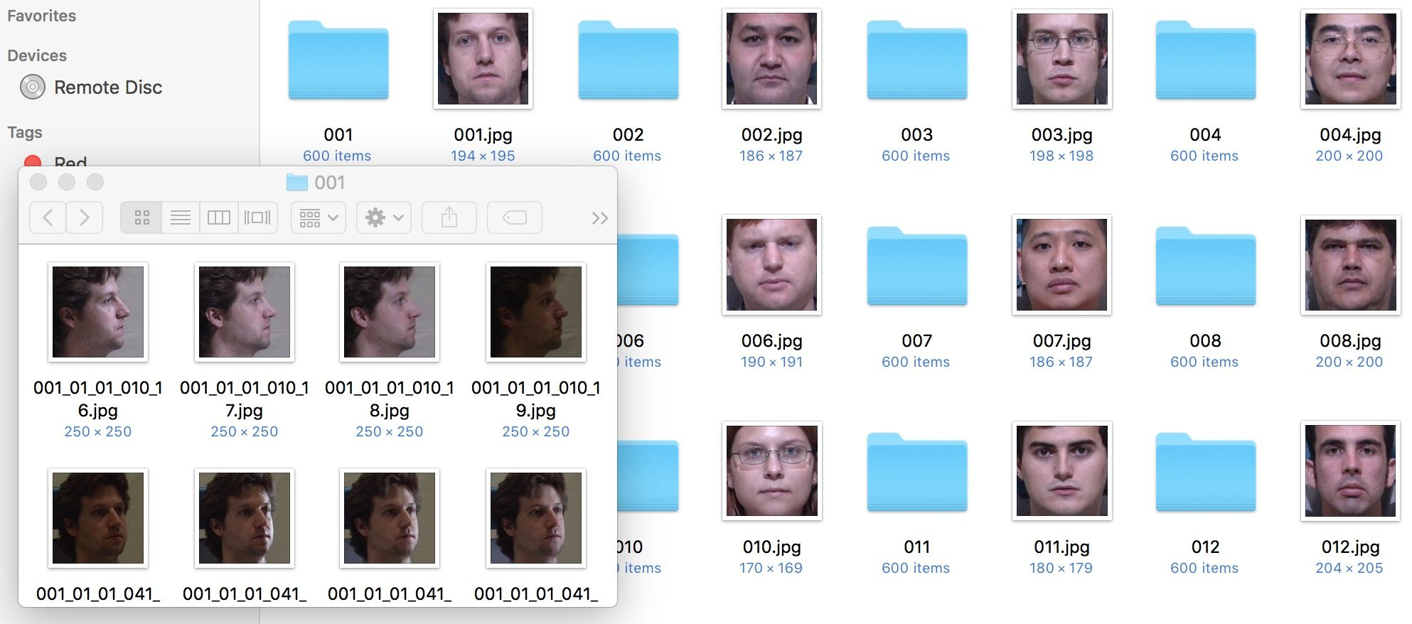
For the face frontalization project, we set up our dataset in the following way: the dataset folder contains a subfolder and a target frontal image for each person (aka subject). In principle, the names of the subfolders and the target images do not have to be identical (as they are in the figure below), but if we are to separately sort all the subfolders and all the targets alphanumerically, the ones corresponding to the same subject must appear at the same position on the two lists of names.
As you can see, subfolder 001/ corresponding to subject 001 contains images of the person pictured in 001.webp — these are closely cropped images of the face under different poses, lighting conditions, and varying face expressions. For the purposes of face frontalization, it is crucial to have the frontal images aligned as close to one another as possible, whereas the other (profile) images have a little bit more leeway.
For instance, our target frontal images are all squares and cropped in such a way that the bottom of the person’s chin is located at the bottom of the image, and the centred point between the inner corners of the eyes is situated at 0.8h above and 0.5h to the right of the lower left corner (h being the image’s height). This way, once the images are resized to 128×128, the face features all appear at more or less the same locations on the images in the training set, and the network can learn to generate the said features and combine them together into realistic synthetic faces.
pipeline:We are now going to build a pipeline for our dataset that is going to inherit from nvidia.dali.pipeline.Pipeline. At the time of writing, DALI does not directly support reading (image, image) pairs from a directory, so we will be making use of nvidia.dali.ops.ExternalSource() to pass the inputs and the targets to the pipeline.
data.pyimport collectionsfrom random import shuffleimport osfrom os import listdirfrom os.path import joinimport numpy as npfrom nvidia.dali.pipeline import Pipelineimport nvidia.dali.ops as ops import nvidia.dali.types as typesdef is.webp(filename): return any(filename.endswith(extension) for extension in [".webp", ".webp"])def get_subdirs(directory): subdirs = sorted([join(directory,name) for name in sorted(os.listdir(directory)) if os.path.isdir(os.path.join(directory, name))]) return subdirsflatten = lambda l: [item for sublist in l for item in sublist]class ExternalInputIterator(object): def __init__(self, imageset_dir, batch_size, random_shuffle=False): self.images_dir = imageset_dir self.batch_size = batch_size # First, figure out what are the inputs and what are the targets in your directory structure: # Get a list of filenames for the target (frontal) images self.frontals = np.array([join(imageset_dir, frontal_file) for frontal_file in sorted(os.listdir(imageset_dir)) if is.webp(frontal_file)]) # Get a list of lists of filenames for the input (profile) images for each person profile_files = [[join(person_dir, profile_file) for profile_file in sorted(os.listdir(person_dir)) if is.webp(profile_file)] for person_dir in get_subdirs(imageset_dir)] # Build a flat list of frontal indices, corresponding to the *flattened* profile_files # The reason we are doing it this way is that we need to keep track of the multiple inputs corresponding to each target frontal_ind = [] for ind, profiles in enumerate(profile_files): frontal_ind += [ind]*len(profiles) self.frontal_indices = np.array(frontal_ind) # Now that we have built frontal_indices, we can flatten profile_files self.profiles = np.array(flatten(profile_files)) # Shuffle the (input, target) pairs if necessary: in practice, it is profiles and frontal_indices that get shuffled if random_shuffle: ind = np.array(range(len(self.frontal_indices))) shuffle(ind) self.profiles = self.profiles[ind] self.frontal_indices = self.frontal_indices[ind] def __iter__(self): self.i = 0 self.n = len(self.frontal_indices) return self # Return a batch of (input, target) pairs def __next__(self): profiles = [] frontals = [] for _ in range(self.batch_size): profile_filename = self.profiles[self.i] frontal_filename = self.frontals[self.frontal_indices[self.i]] profile = open(profile_filename, 'rb') frontal = open(frontal_filename, 'rb') profiles.append(np.frombuffer(profile.read(), dtype = np.uint8)) frontals.append(np.frombuffer(frontal.read(), dtype = np.uint8)) profile.close() frontal.close() self.i = (self.i + 1) % self.n return (profiles, frontals) next = __next__class ImagePipeline(Pipeline): ''' Constructor arguments: - imageset_dir: directory containing the dataset - image_size = 128: length of the square that the images will be resized to - random_shuffle = False - batch_size = 64 - num_threads = 2 - device_id = 0 ''' def __init__(self, imageset_dir, image_size=128, random_shuffle=False, batch_size=64, num_threads=2, device_id=0): super(ImagePipeline, self).__init__(batch_size, num_threads, device_id, seed=12) eii = ExternalInputIterator(imageset_dir, batch_size, random_shuffle) self.iterator = iter(eii) self.num_inputs = len(eii.frontal_indices) # The source for the inputs and targets self.input = ops.ExternalSource() self.target = ops.ExternalSource() # n.webpDecoder below accepts CPU inputs, but returns GPU outputs (hence device = "mixed") self.decode = ops.n.webpDecoder(device = "mixed", output_type = types.RGB) # The rest of pre-processing is done on the GPU self.res = ops.Resize(device="gpu", resize_x=image_size, resize_y=image_size) self.norm = ops.NormalizePermute(device="gpu", output_dtype=types.FLOAT, mean=[128., 128., 128.], std=[128., 128., 128.], height=image_size, width=image_size) # epoch_size = number of (profile, frontal) image pairs in the dataset def epoch_size(self, name = None): return self.num_inputs # Define the flow of the data loading and pre-processing def define_graph(self): self.profiles = self.input(name="inputs") self.frontals = self.target(name="targets") profile_images = self.decode(self.profiles) profile_images = self.res(profile_images) profile_output = self.norm(profile_images) frontal_images = self.decode(self.frontals) frontal_images = self.res(frontal_images) frontal_output = self.norm(frontal_images) return (profile_output, frontal_output) def iter_setup(self): (images, targets) = self.iterator.next() self.feed_input(self.profiles, images) self.feed_input(self.frontals, targets)You can now use the ImagePipeline class that you wrote above to load images from your dataset directory, one batch at a time.
If you are using the code from this tutorial inside a Jupyter notebook, here is how you can use an ImagePipeline to display the images:
from __future__ import divisionimport matplotlib.gridspec as gridspecimport matplotlib.pyplot as plt%matplotlib inlinedef show_images(image_batch, batch_size): columns = 4 rows = (batch_size + 1) // (columns) fig = plt.figure(figsize = (32,(32 // columns) * rows)) gs = gridspec.GridSpec(rows, columns) for j in range(rows*columns): plt.subplot(gs[j]) plt.axis("off") plt.imshow(np.transpose(image_batch.at(j), (1,2,0)))batch_size = 8pipe = ImagePipeline('my_dataset_directory', image_size=128, batch_size=batch_size)pipe.build()profiles, frontals = pipe.run()# The images returned by ImagePipeline are currently on the GPU# We need to copy them to the CPU via the asCPU() method in order to display themshow_images(profiles.asCPU(), batch_size=batch_size)show_images(frontals.asCPU(), batch_size=batch_size)Here comes the fun part, building the network’s architecture! We assume that you are already somewhat familiar with the idea behind convolutional neural networks, the architecture of choice for many computer vision applications today.
Beyond that, there are two main concepts that we will need for the face Frontalization project, that we shall touch upon in this section:
The Encoder
As mentioned above, our network takes images that are sized 128 by 128 as input. Since the images are in colour (meaning 3 colour channels for each pixel), this results in the input being 3 × 128 × 128 = 49152 dimensional. Perhaps we do not need all 49152 values to describe a person’s face? This turns out to be correct: we can get away with a mere 512 dimensional vector (which is simply another way of saying “512 numbers”) to encode all the information that we care about. This is an example of dimensionality reduction: the Encoder network (paired with the network responsible for the inverse process, decoding) learns a lower dimensional representation of the input. The architecture of the Encoder may look something like this:
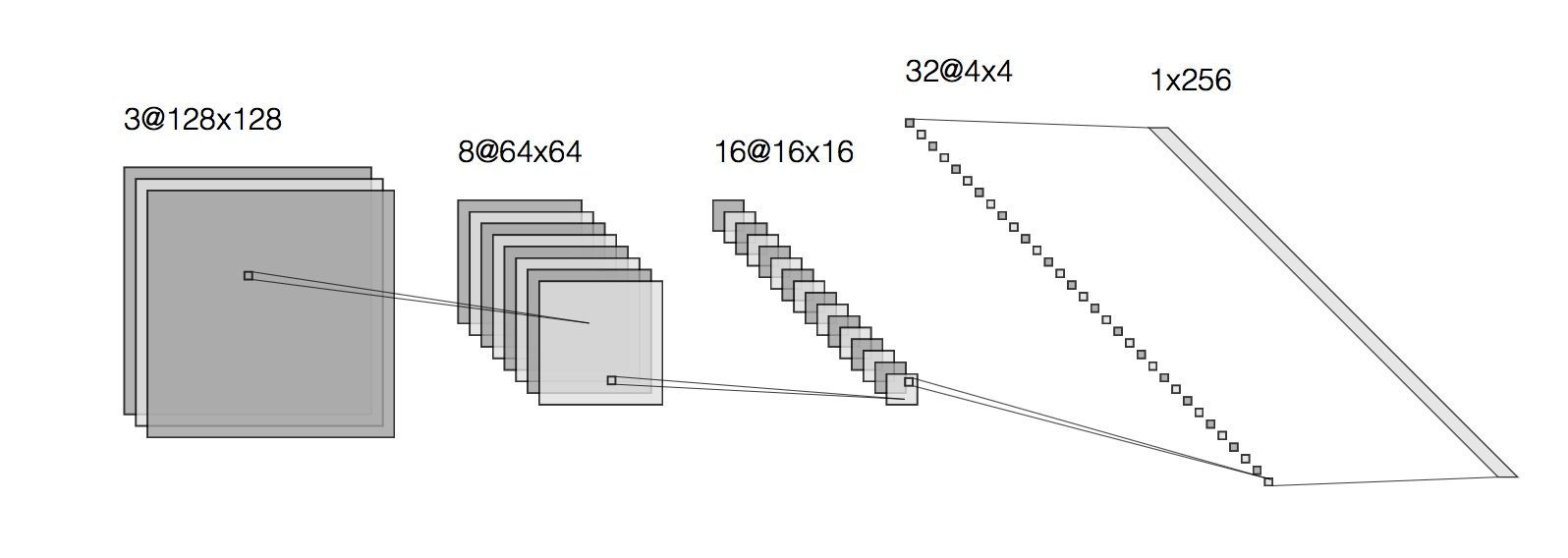
Here we start with input that is 128×128 and has 3 channels. As we pass it through convolutional layers, the size of the input gets smaller and smaller (from 128×128 to 64×64 to 16×16 etc on the figure above) whereas the number of channels grows (from 3 to 8 to 16 and so on). This reflects the fact that the deeper the convolutional layer, the more abstract are the features that it learns. In the end we get to a layer whose output is sized 1×1, yet has a very high number of channels: 256 in the example depicted above (or 512 in our own network). 256×1 and 1×256 are really the same thing, if you think about it, so another way to put it is that the output of the Encoder is 256 dimensional (with a single channel), so we have reduced the dimensionality of the original input from 49152 to 256! Why would we want to do that? Having this lower dimensional representation helps us prevent overfitting our final model to the training set.
In the end, what we want is a representation (and hence, a model) that is precise enough to fit the training data well, yet does not overfit — meaning, that it can be generalised to the data it has not seen before as well.
The Decoder
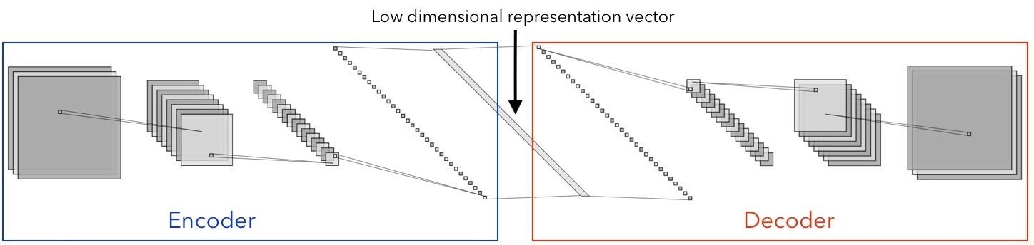
As the name suggests, the Decoder’s job is the inverse of that of the Encoder. In other words, it takes the low-dimensional representation output of the Encoder and has it go through deconvolutional layers (also known as the transposed convolutional layers). The architecture of the Decoder network is often symmetric to that of the Encoder, although this does not have to be the case. The Encoder and the Decoder are often combined into a single network, whose inputs and outputs are both images:
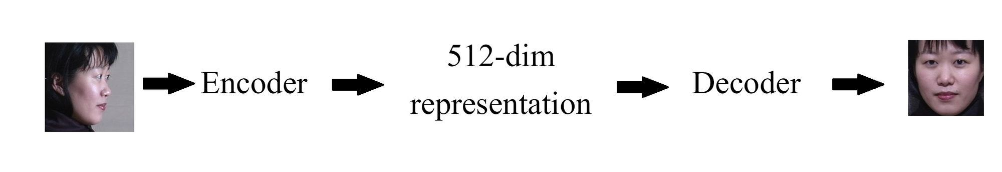
In our project this Encoder/Decoder network is called the Generator. The Generator takes in a profile image, and (if we do our job right) outputs a frontal one:
It is now time to write it using PyTorch. A two dimensional convolutional layer can be created via torch.nn.Conv2d(in_channels, out_channels, kernel_size, stride, padding). You can now read off the architecture of our Generator network from the code snippet below:
network.pyimport torchimport torch.nn as nnimport torch.nn.parallelimport torch.optim as optimfrom torch.autograd import Variabledef weights_init(m): classname = m.__class__.__name__ if classname.find('Conv') != -1: m.weight.data.normal_(0.0, 0.02) elif classname.find('BatchNorm') != -1: m.weight.data.normal_(1.0, 0.02) m.bias.data.fill_(0)''' Generator network for 128x128 RGB images '''class G(nn.Module): def __init__(self): super(G, self).__init__() self.main = nn.Sequential( # Input HxW = 128x128 nn.Conv2d(3, 16, 4, 2, 1), # Output HxW = 64x64 nn.BatchNorm2d(16), nn.ReLU(True), nn.Conv2d(16, 32, 4, 2, 1), # Output HxW = 32x32 nn.BatchNorm2d(32), nn.ReLU(True), nn.Conv2d(32, 64, 4, 2, 1), # Output HxW = 16x16 nn.BatchNorm2d(64), nn.ReLU(True), nn.Conv2d(64, 128, 4, 2, 1), # Output HxW = 8x8 nn.BatchNorm2d(128), nn.ReLU(True), nn.Conv2d(128, 256, 4, 2, 1), # Output HxW = 4x4 nn.BatchNorm2d(256), nn.ReLU(True), nn.Conv2d(256, 512, 4, 2, 1), # Output HxW = 2x2 nn.MaxPool2d((2,2)), # At this point, we arrive at our low D representation vector, which is 512 dimensional. nn.ConvTranspose2d(512, 256, 4, 1, 0, bias = False), # Output HxW = 4x4 nn.BatchNorm2d(256), nn.ReLU(True), nn.ConvTranspose2d(256, 128, 4, 2, 1, bias = False), # Output HxW = 8x8 nn.BatchNorm2d(128), nn.ReLU(True), nn.ConvTranspose2d(128, 64, 4, 2, 1, bias = False), # Output HxW = 16x16 nn.BatchNorm2d(64), nn.ReLU(True), nn.ConvTranspose2d(64, 32, 4, 2, 1, bias = False), # Output HxW = 32x32 nn.BatchNorm2d(32), nn.ReLU(True), nn.ConvTranspose2d(32, 16, 4, 2, 1, bias = False), # Output HxW = 64x64 nn.BatchNorm2d(16), nn.ReLU(True), nn.ConvTranspose2d(16, 3, 4, 2, 1, bias = False), # Output HxW = 128x128 nn.Tanh() ) def forward(self, input): output = self.main(input) return outputGenerative Adversarial Networks (GANs) are a very exciting deep learning development, which was introduced in a 2014 paper by Ian Goodfellow and collaborators. Without getting into too much detail, here is the idea behind GANs: there are two networks, a Generator (perhaps our name choice for the Encoder/Decoder net above makes more sense now) and a Discriminator. The Generator’s job is to generate synthetic images, but what is the Discriminator to do? The Discriminator is supposed to tell the difference between the real images and the fake ones that were synthesised by the Generator.
Usually, GAN training is carried out in an unsupervised manner. There is an unlabelled dataset of, say, images in a specific domain. The Generator will generate some image given random noise as input. The Discriminator is then trained to recognise the images from the dataset as real and the output of the Generator as fake. As far as the Discriminator is concerned, the two categories comprise a labelled dataset. If this sounds like a binary classification problem to you, you won’t be surprised to hear that the loss function is the binary cross entropy. The task of the generator is to fool the Discriminator. Here is how that is done: first, the generator gives its output to the Discriminator. Naturally, that output depends on what the generator’s trainable parameters are. The Discriminator is not being trained at this point, rather it is used for inference. Instead, it is the _Generator’_s weights that are updated in a way that gets the Discriminator to accept (as in, label as “real”) the synthesised outputs. The updating of the Generator’s and the discriminator’s weights is done alternatively — once each for every batch, as you will see later when we discuss training our model.
Since we are not trying to simply generate faces, the architecture of our Generator is a little different from the one described above (for one thing, it takes real images as inputs, not some random noise, and tries to incorporate certain features of those inputs in its outputs). Our loss function won’t be just the cross-entropy either: we have to add an additional component that compares the generator’s outputs to the target ones. This could be, for instance, a pixelwise mean square error, or a mean absolute error. These matters are going to be addressed in the Training section of this tutorial.
Before we move on, let us complete the network.py file by providing the code for the Discriminator:
network.py [continued]''' Discriminator network for 128x128 RGB images '''class D(nn.Module): def __init__(self): super(D, self).__init__() self.main = nn.Sequential( nn.Conv2d(3, 16, 4, 2, 1), nn.LeakyReLU(0.2, inplace = True), nn.Conv2d(16, 32, 4, 2, 1), nn.BatchNorm2d(32), nn.LeakyReLU(0.2, inplace = True), nn.Conv2d(32, 64, 4, 2, 1), nn.BatchNorm2d(64), nn.LeakyReLU(0.2, inplace = True), nn.Conv2d(64, 128, 4, 2, 1), nn.BatchNorm2d(128), nn.LeakyReLU(0.2, inplace = True), nn.Conv2d(128, 256, 4, 2, 1), nn.BatchNorm2d(256), nn.LeakyReLU(0.2, inplace = True), nn.Conv2d(256, 512, 4, 2, 1), nn.BatchNorm2d(512), nn.LeakyReLU(0.2, inplace = True), nn.Conv2d(512, 1, 4, 2, 1, bias = False), nn.Sigmoid() ) def forward(self, input): output = self.main(input) return output.view(-1)As you can see, the architecture of the Discriminator is rather similar to that of the Generator, except that it seems to contain only the Encoder part of the latter. Indeed, the goal of the Discriminator is not to output an image, so there is no need for something like a Decoder. Instead, the Discriminator contains layers that process an input image (much like an Encoder would), with the goal of distinguishing real images from the synthetic ones.
DALI is a wonderful tool that not only pre-processes images on the fly, but also provides plugins for several popular machine learning frameworks, including PyTorch.
If you used PyTorch before, you may be familiar with its torch.utils.data.Dataset and torch.utils.data.DataLoader classes meant to ease the pre-processing and loading of the data. When using DALI, we combine the aforementioned nvidia.dali.pipeline.Pipeline with nvidia.dali.plugin.pytorch.DALIGenericIterator in order to accomplish the task.
At this point, we are starting to get into the third Python file that is a part of the face frontalization project. First, let us get the imports out of the way. We’ll also set the seeds for the randomised parts of our model in order to have better control over reproducibility of the results:
main.pyfrom __future__ import print_functionimport timeimport mathimport randomimport osfrom os import listdirfrom os.path import joinfrom PIL import Imageimport numpy as npimport torchimport torch.nn as nnimport torch.nn.parallelimport torch.optim as optimimport torchvision.utils as vutilsfrom torch.autograd import Variablefrom nvidia.dali.plugin.pytorch import DALIGenericIteratorfrom data import ImagePipelineimport networknp.random.seed(42)random.seed(10)torch.backends.cudnn.deterministic = Truetorch.backends.cudnn.benchmark = Falsetorch.manual_seed(999)# Where is your training dataset at?datapath = 'training_set'# You can also choose which GPU you want your model to be trained on below:gpu_id = 0device = torch.device("cuda", gpu_id)In order to integrate the ImagePipeline class from data.py into your PyTorch model, you will need to make use of DALIGenericIterator. Constructing one is very straightforward: you only need to pass it a pipeline object, a list of labels for what your pipeline spits out, and the epoch_size of the pipeline. Here is what that looks like:
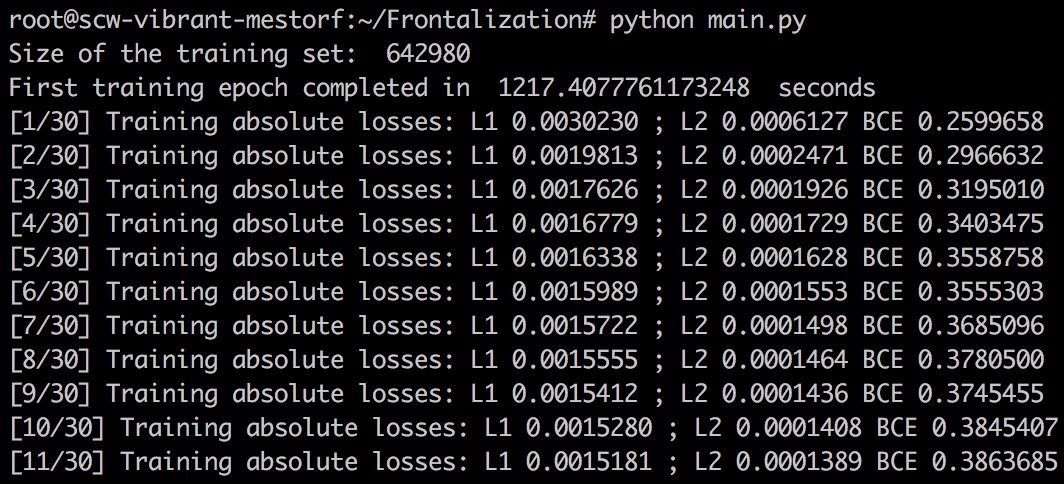
main.py [continued]train_pipe = ImagePipeline(datapath, image_size=128, random_shuffle=True, batch_size=30, device_id=gpu_id)train_pipe.build()m_train = train_pipe.epoch_size()print("Size of the training set: ", m_train)train_pipe_loader = DALIGenericIterator(train_pipe, ["profiles", "frontals"], m_train)Now you are ready to train.
First, lets get ourselves some neural networks:
main.py [continued]# Generator:netG = network.G().to(device)netG.apply(network.weights_init)# Discriminator:netD = network.D().to(device)netD.apply(network.weights_init)Mathematically, training a neural network refers to updating its weights in a way that minimises the loss function. There are multiple choices to be made here, the most crucial, perhaps, being the form of the loss function. We have already touched upon it in our discussion of GANs in Step 3, so we know that we need the binary cross entropy loss for the discriminator, whose job is to classify the images as either real or fake.
However, we also want a pixelwise loss function that will get the generated outputs to not only look like frontal images of people in general, but the right people - same ones that we see in the input profile images. The common ones to use are the so-called L1 loss and L2 loss: you might know them under the names of Mean Absolute Error and Mean Squared Error respectively. In the code below, we’ll give you both (in addition to the cross entropy), together with a way to vary the relative importance you place on each of the three.
main.py [continued]# Here is where you set how important each component of the loss function is:L1_factor = 0L2_factor = 1GAN_factor = 0.0005criterion = nn.BCELoss() # Binary cross entropy loss# Optimizers for the generator and the discriminator (Adam is a fancier version of gradient descent with a few more bells and whistles that is used very often):optimizerD = optim.Adam(netD.parameters(), lr = 0.0002, betas = (0.5, 0.999))optimizerG = optim.Adam(netG.parameters(), lr = 0.0002, betas = (0.5, 0.999), eps = 1e-8)# Create a directory for the output filestry: os.mkdir('output')except OSError: passstart_time = time.time()# Let's train for 30 epochs (meaning, we go through the entire training set 30 times):for epoch in range(30): # Lets keep track of the loss values for each epoch: loss_L1 = 0 loss_L2 = 0 loss_gan = 0 # Your train_pipe_loader will load the images one batch at a time # The inner loop iterates over those batches: for i, data in enumerate(train_pipe_loader, 0): # These are your images from the current batch: profile = data[0]['profiles'] frontal = data[0]['frontals'] # TRAINING THE DISCRIMINATOR netD.zero_grad() real = Variable(frontal).type('torch.FloatTensor').to(device) target = Variable(torch.ones(real.size()[0])).to(device) output = netD(real) # D should accept the GT images errD_real = criterion(output, target) profile = Variable(profile).type('torch.FloatTensor').to(device) generated = netG(profile) target = Variable(torch.zeros(real.size()[0])).to(device) output = netD(generated.detach()) # detach() because we are not training G here # D should reject the synthetic images errD_fake = criterion(output, target) errD = errD_real + errD_fake errD.backward() # Update D optimizerD.step() # TRAINING THE GENERATOR netG.zero_grad() target = Variable(torch.ones(real.size()[0])).to(device) output = netD(generated) # G wants to : # (a) have the synthetic images be accepted by D (= look like frontal images of people) errG_GAN = criterion(output, target) # (b) have the synthetic images resemble the ground truth frontal image errG_L1 = torch.mean(torch.abs(real - generated)) errG_L2 = torch.mean(torch.pow((real - generated), 2)) errG = GAN_factor * errG_GAN + L1_factor * errG_L1 + L2_factor * errG_L2 loss_L1 += errG_L1.item() loss_L2 += errG_L2.item() loss_gan += errG_GAN.item() errG.backward() # Update G optimizerG.step() if epoch == 0: print('First training epoch completed in ',(time.time() - start_time),' seconds') # reset the DALI iterator train_pipe_loader.reset() # Print the absolute values of three losses to screen: print('[%d/30] Training absolute losses: L1 %.7f ; L2 %.7f BCE %.7f' % ((epoch + 1), loss_L1/m_train, loss_L2/m_train, loss_gan/m_train,)) # Save the inputs, outputs, and ground truth frontals to files: vutils.save_image(profile.data, 'output/%03d_input.webp' % epoch, normalize=True) vutils.save_image(real.data, 'output/%03d_real.webp' % epoch, normalize=True) vutils.save_image(generated.data, 'output/%03d_generated.webp' % epoch, normalize=True) # Save the pre-trained Generator as well torch.save(netG,'output/netG_%d.pt' % epoch)Training GANs is notoriously difficult, but let us focus on the L2 loss, equal to the sum of squared differences between each pixel of the output and target images. Its value decreases with every epoch, and if we compare the generated images to the real ones of frontal faces, we see that our model is indeed learning to fit the training data:
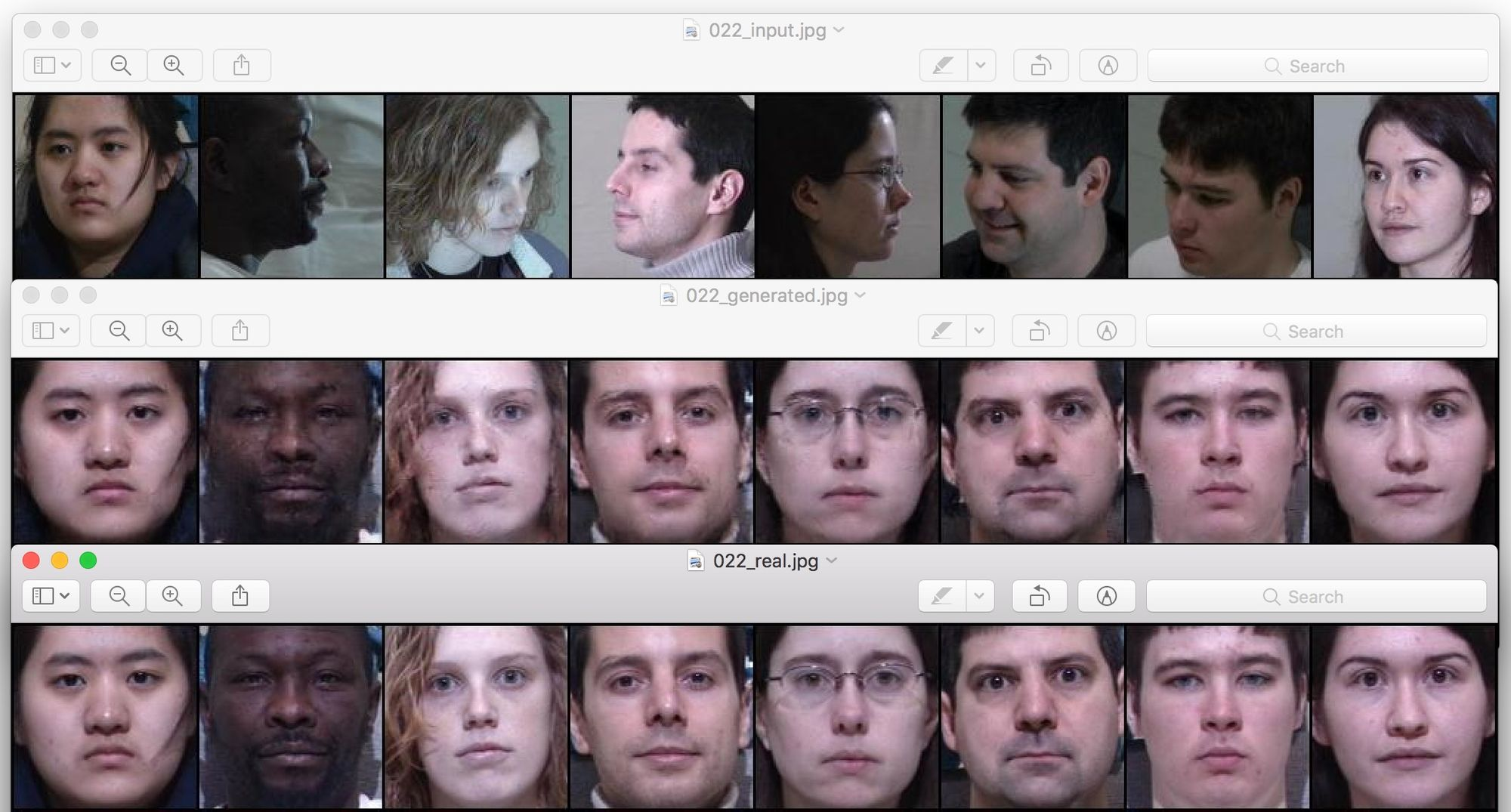
In the figure above, the upper row are some of the inputs fed into our model during the 22nd training epoch, below are the frontal images generated by our GAN, and at the bottom is the row of the corresponding ground truth images.
Next, lets see how the model performs on data that it has never seen before.
We are going to test the model we trained in the previous section on the three subjects that appear in the comparison table in the paper Beyond Face Rotation: Global and Local Perception GAN for Photorealistic and Identity Preserving Frontal View Synthesis. These subjects do not appear in our training set; instead, we put the corresponding images in a directory called test_set that has the same structure as the training_set above. The test.py code is going to load a pre-trained generator network that we saved during training, and put the input test images through it, generating the outputs:
test.pyimport torchimport torchvision.utils as vutilsfrom torch.autograd import Variablefrom nvidia.dali.plugin.pytorch import DALIGenericIteratorfrom data import ImagePipelinedevice = 'cuda'datapath = 'test_set'# Generate frontal images from the test setdef frontalize(model, datapath, mtest): test_pipe = ImagePipeline(datapath, image_size=128, random_shuffle=False, batch_size=mtest) test_pipe.build() test_pipe_loader = DALIGenericIterator(test_pipe, ["profiles", "frontals"], mtest) with torch.no_grad(): for data in test_pipe_loader: profile = data[0]['profiles'] frontal = data[0]['frontals'] generated = model(Variable(profile.type('torch.FloatTensor').to(device))) vutils.save_image(torch.cat((profile, generated.data, frontal)), 'output/test.webp', nrow=mtest, padding=2, normalize=True) return# Load a pre-trained Pytorch modelsaved_model = torch.load("./output/netG_15.pt")frontalize(saved_model, datapath, 3)Here are the results of the model above that has been trained for 15 epochs:
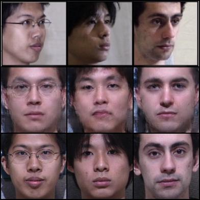
Again, here we see input images on top, followed by generated images in the middle and the ground truth ones at the bottom. Naturally, the agreement between the latter two is not as close as that for the images in the training set, yet we see that the network did in fact learn to pick up various facial features such as glasses, thickness of the eyebrows, eye and nose shape etc. In the end, one has to experiment with the hyperparameters of the model to see what works best. We managed to produce the following results in just five training epochs (which take about an hour and a half on the Scaleway RENDER-S GPU Instances):
| Input |  |
|---|---|
| Generated output |  |
Here we have trained the GAN model with parameters as in the code above for the first three epochs, then set the GAN_factor to zero and continued to train only the generator, optimizing the L2 loss, for two more epochs.
For any science fiction fan, Deep Learning is a dream come true: this rapidly growing field of Artificial Intelligence lies at the heart of many technologies previously thought to be impossible. Face frontalization is only one example, and as we demonstrate in this article, many of the projects at today’s AI research frontier can be implemented with the resources available to the general public. So do not wait to start your own journey into Deep Learning, sign up for a GPU Instance on Scaleway today and get coding!
We will take a detailed look at the Variational Autoencoder: a generative model based on its more commonplace sibling, the Autoencoder (which we will devote some time to below as well).

You have just spent weeks developing your new machine learning model, you are finally happy enough with its performance, and you want to show it off to the rest of the world.

In this article, we will talk about active learning and how to apply the concepts to an image classification task with PyTorch.