Achieving Super-Resolution with a Sub-Pixel Convolutional Neural Network on Scaleway GPU

Reviewed on 03 October 2024 • Published on 24 September 2020

Scaleway-GPU
AI
inference
Super-Resolution

Super-resolution is the process of enhancing the details of a low-resolution image to recover a high-resolution image. In the context of deep learning, the technique consists of taking a low-resolution image as input, passing it through a neural network, and receiving an output that is a higher-resolution version of the input.

The neural network upscales the image by filling in the finer details based on the knowledge it obtained in the training process.

One of the ways to train a model is to use a training dataset. It consists of downscaling high-resolution images as the input and the high-resolution images themselves as the output. This method is also known as the ground truth.

After the model has been trained, a separate test set should be used to guarantee the model’s performance on images that were not part of the initial dataset.

In this tutorial, we will show you how to prepare your data, construct the sub-pixel convolutional neural network, train it, and test it using a Scaleway GPU instance.

Before you start

To complete the actions presented below, you must have:

A Scaleway account logged into the console
Owner status or IAM permissions allowing you to perform actions in the intended Organization
A GPU Instance running on UbuntuML
Configured Jupyter Notebook on your GPU Instance
sudo privileges or access to the root user

Preparing the data

Import the training set from your local machine to your remote Instance directory, before you begin setting up your data pipeline. You can use scp to do so, with the following command:

Note

We assume that you have previously created train and test directories within the directory being transferred.

scp -r <path-localhost> root@<host>:<path-remotehost>/

Important

Replace <path-localhost> with the path to the directory you dataset is located in your local host. In root@<host> replace <host> with your remote GPU instance’s IP address. <path-remotehost> should be replaced with the path you wish to save your datasets in your GPU Instance.

Open a Jupyter Notebook to begin setting up your data.

Copy and paste the following code.

To import the libraries:

from __future__ import print_function, division
import time
import os
import numpy as np
import matplotlib.pyplot as plt
from PIL import Image
import torch
import torch.nn as nn
import torch.optim as optim
from torch.autograd import Variable
from torch.utils.data import Dataset, DataLoader
from torchvision import transforms, utils
import torchvision
device = 'cuda' if torch.cuda.is_available() else 'cpu'
# The Super Resolution model will work for images of arbitrary size, but will
# be optimized for images with dimensions equal to:
image_size = 60
# The factor by which the image size should increase after Super Resolution:
scaleup = 2

To set directory paths for the training and test data sets. Replace ./Path/train with the path to your training dataset and ./Path/test with the path to the testing dataset.

# Set directory paths for the training and test data sets:
# the directories' structure does not matter, as long as they contain image files
traindir = './Path/train'
testdir = './Path/test/'

# For best performance, only images whose original size is at least image_size x scaleup
# will be included in the training set. This will be checked here:
def is_good_image(filename, min_dim):
    if any(filename.endswith(extension) for extension in [".webp", ".jpeg"]):
        image = Image.open(filename)
        return(min(image.size) >= min_dim)
    return False
# Display the torch tensor as image with figsize = size
def show(torch_tensor, size=(4,4)):
    npimg = torch_tensor.numpy()
    plt.figure(figsize = size)
    plt.imshow(np.transpose(npimg, (1,2,0)))
    plt.show()
'''
    Custom PyTorch dataset class that inherits torch.utils.data.Dataset
    Each instance of the ResolutionDataset is a pair of images:
    - an image of size lowres x lowres
    - the same image but of size lowres*upscale x lowres*upscale
'''
  class ResolutionDataset(Dataset):
    def __init__(self, root_dir, lowres = image_size, upscale = scaleup):
        list_files = list()
        for (dirpath, dirnames, filenames) in os.walk(root_dir):
            list_files += [os.path.join(dirpath, file) for file in filenames if is_good_image(os.path.join(dirpath, file), upscale*lowres)]
        self.image_files = np.asarray(list_files)
        self.lowres = lowres
        self.upscale = upscale
    def __len__(self):
        return len(self.image_files)
    def __getitem__(self, idx):
        if torch.is_tensor(idx):
            idx = idx.tolist()
        image = Image.open(self.image_files[idx])
        transform_LR = transforms.Compose([transforms.CenterCrop(min(image.size)),
                                          transforms.Resize(self.lowres), transforms.ToTensor()])
        image_LR = transform_LR(image)
        transform_HR = transforms.Compose([transforms.CenterCrop(min(image.size)),
                                          transforms.Resize(self.lowres*self.upscale), transforms.ToTensor()])
        image_HR = transform_HR(image)
        return image_LR, image_HR

Note

If you want to know more about creating custom Python dataset classes, refer to the Pytorch “Writing Custom Datasets, Dataloaders and Transforms” tutorial.

trainset = ResolutionDataset(traindir)
testset = ResolutionDataset(testdir)
dataloader = DataLoader(trainset, batch_size=128, shuffle=True, num_workers=10)
testloader = DataLoader(testset, batch_size=128, shuffle=False)

Constructing the network

'''
    The Super Resolution model from the Sub-Pixel Convolutional Neural Network paper
    (https://www.cv-foundation.org/openaccess/content_cvpr_2016/papers/Shi_Real-Time_Single_Image_CVPR_2016_paper.pdf)
    upscale_factor = factor by which the image size should increase after Super Resolution
'''
class SubPixelNetwork(nn.Module):
    def __init__(self, upscale_factor):
        super(SubPixelNetwork, self).__init__()
        self.relu = nn.ReLU()
        self.conv1 = nn.Conv2d(3, 64, (5, 5), (1, 1), (2, 2))
        self.conv2 = nn.Conv2d(64, 64, (3, 3), (1, 1), (1, 1))
        self.conv3 = nn.Conv2d(64, 32, (3, 3), (1, 1), (1, 1))
        self.conv4 = nn.Conv2d(32, (upscale_factor ** 2)*3, (3, 3), (1, 1), (1, 1))
        # Sub-pixel convolution: rearranges elements in a Tensor of shape (*, r^2C, H, W)
        # to a tensor of shape (C, rH, rW)
        self.pixel_shuffle = nn.PixelShuffle(upscale_factor)
        self._initialize_weights()
    def forward(self, x):
        x = self.relu(self.conv1(x))
        x = self.relu(self.conv2(x))
        x = self.relu(self.conv3(x))
        x = self.pixel_shuffle(self.conv4(x))
        return x
    def _initialize_weights(self):
        nn.init.orthogonal_(self.conv1.weight, nn.init.calculate_gain('relu'))
        nn.init.orthogonal_(self.conv2.weight, nn.init.calculate_gain('relu'))
        nn.init.orthogonal_(self.conv3.weight, nn.init.calculate_gain('relu'))
        nn.init.orthogonal_(self.conv4.weight)

model = SubPixelNetwork(scaleup).to(device)
optimizer = optim.Adam(model.parameters(), lr=0.001)

Training and testing the network

'''
    Train the model for one epoch
    - model
    - optimizer
    - dataloader: torch.utils.data.DataLoader with the training data
    - device: cpu or gpu
'''
def train(model, optimizer, dataloader, device):
    epoch_loss = 0
    for i, data in enumerate(dataloader):
        optimizer.zero_grad()
        inputs = data[0].type('torch.FloatTensor').to(device)
        targets = data[1].type('torch.FloatTensor').to(device)
        outputs = model(inputs)
        # L2 loss (pixelwise mean error squared)
        loss = torch.mean(torch.pow((targets - outputs), 2))
        epoch_loss += loss.item()
        loss.backward()
        optimizer.step()
    return epoch_loss
'''
    Run the model on the test set
    - model
    - testloader: torch.utils.data.DataLoader with the test data
    - device: cpu or gpu
    - display: when set to True, the last batch of the testloader gets printed to screen
    (the low res inputs, model's outputs, followed by the ground truth images)
'''
def test(model, testloader, device, display=False):
    epoch_loss = 0
    for i, data in enumerate(testloader):
        inputs = data[0].type('torch.FloatTensor').to(device)
        targets = data[1].type('torch.FloatTensor').to(device)
        with torch.no_grad():
            outputs = model(inputs)
            loss = torch.mean(torch.pow((targets - outputs), 2))
            epoch_loss += loss.item()
    if display:
        # Display the inputs, outputs and targets from the last batch:
        b_size = inputs.size()[0]
        inputs = torchvision.utils.make_grid(inputs, nrow=b_size, normalize=True)
        outputs = torchvision.utils.make_grid(outputs, nrow=b_size, normalize=True)
        targets = torchvision.utils.make_grid(targets, nrow=b_size, normalize=True)
        show(inputs.cpu(), size=(20,4))
        show(outputs.cpu(), size=(20,4))
        show(targets.cpu(), size=(20,4))
    return epoch_loss

train_losses = []
test_losses = []

Note

You can add train_losses = [] and test_losses = [] so that you can keep track of the loss values during the training and plot them once it is completed.

num_epochs = 20
for epoch in range(num_epochs):
    print(epoch)
    train_loss = train(model, optimizer, dataloader, device)
    train_losses.append(train_loss)
    test_loss = test(model, testloader, device, display=False)
    test_losses.append(test_loss)
fig, ax1 = plt.subplots()
color = 'tab:red'
ax1.set_xlabel('epochs')
ax1.set_ylabel('Train Loss', color=color)
ax1.plot(range(1, num_epochs+1), np.array(train_losses), color=color)
ax1.tick_params(axis='y', labelcolor=color)
ax2 = ax1.twinx()
color = 'tab:blue'
ax2.set_ylabel('Test Loss', color=color)
ax2.plot(range(1, num_epochs+1), np.array(test_losses), color=color)
ax2.tick_params(axis='y', labelcolor=color)
fig.tight_layout()
plt.show()

Results

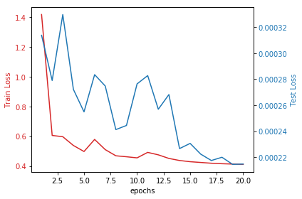
In the plot, you can see the train loss and test loss as a function of training epochs.

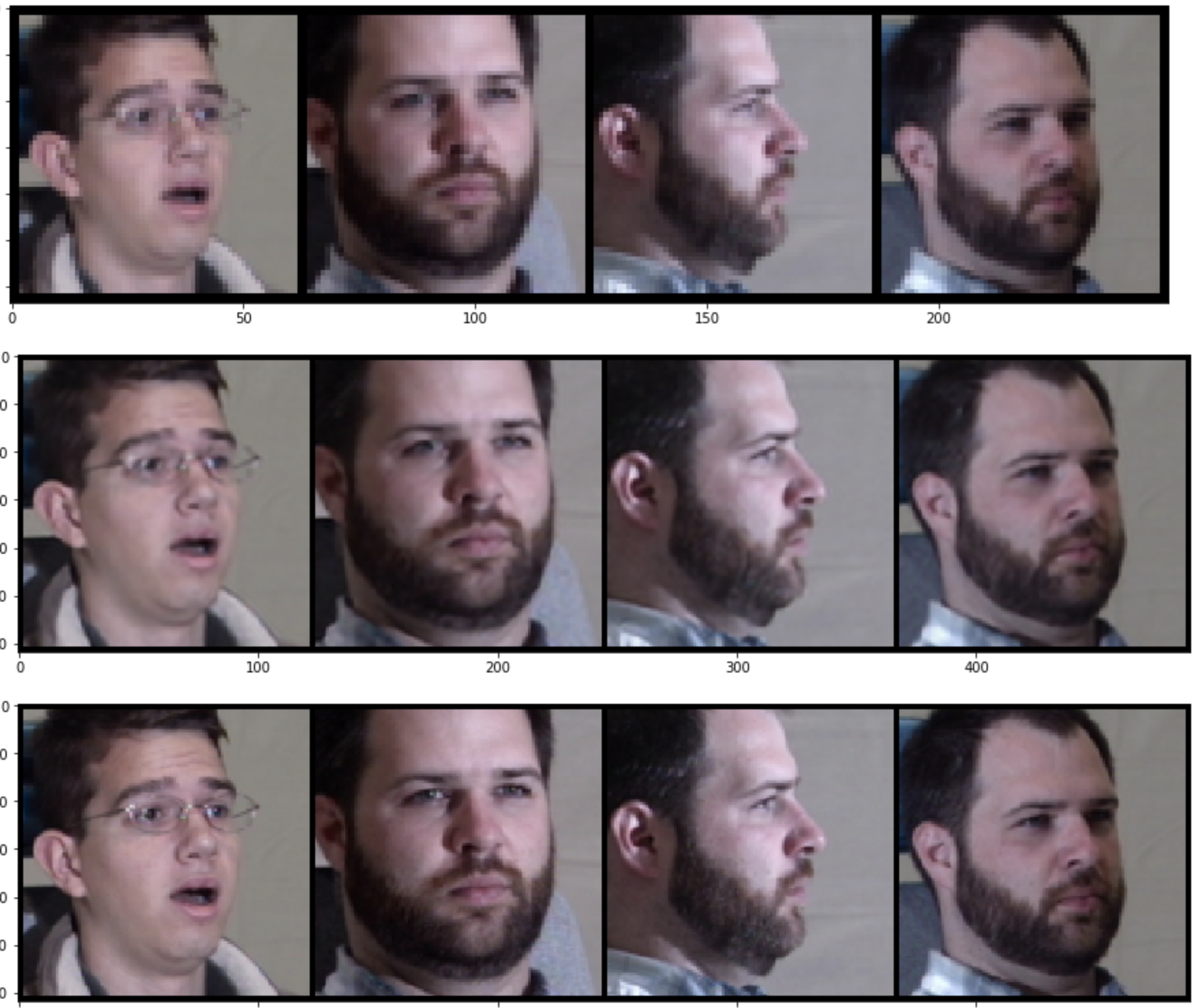
In the image below you can see the results of the Super Resolution:

Upper row: low-resolution inputs
Middle row: model’s super-resolved outputs
Bottom row: the ground truth high-resolution images

To know more about the model used in this tutorial, refer to The Super Resolution model from the Sub-Pixel Convolutional Neural Network paper.